
Visualizing electronegativity of the elements in 3D
While teaching the history and patterns of the periodic table of the elements to my chemistry students, I wanted them to get a better feel for the concept of periodicity – that some elemental properties repeat periodically as you increase atomic numbers.

Melting points of the elements visualized in 3D
For example, at the left of each period (row) is an element that is a soft metal that will react with water to produce a strong base. As a family they are called the alkali metals, and consist of lithium, sodium, potassium, rubidium, cesium, and francium. We now know they have a similar electron configuration, with a single electron in an s-type orbital. This electron is easily ionized away and accounts for the alkali metals’ high reactivity. Other families of elements (usually found in columns in the table) include the noble gases, the halogens, and the royal metals (copper, silver, and gold). It was the relationships of similar properties that led Mendelyev (and de Chancourtois, Newlands, Oddling, and Meyer) to develop the periodic table in the first place.

Melting points with a golden texture
In an effort to visualize these patterns more clearly, I have devised a technique for taking the numerical values of a property, such as electronegativity, atomic radius, or melting point and turning them into three-dimensional models.

Chart for recording the numerical values of a periodic property
I start with a chart that is divided into squares in the shape of the periodic table, with white squares representing elements and black squares the spaces between and around the sections of the table (you can download this diagram here).
Periodic Properties Chart: 3D periodic properties table
Pairs of students look up one of the periodic properties, then write the numbers down for each element on the chart.
In a text editing program such as Text Edit or Microsoft Word, my students then type in the numbers for each row of the chart, separating them by commas and hitting return or enter to make the next row. For the black squares, they type in a zero. They have to be careful not to leave any element or blank square out. They will have 12 rows of 20 numbers each.
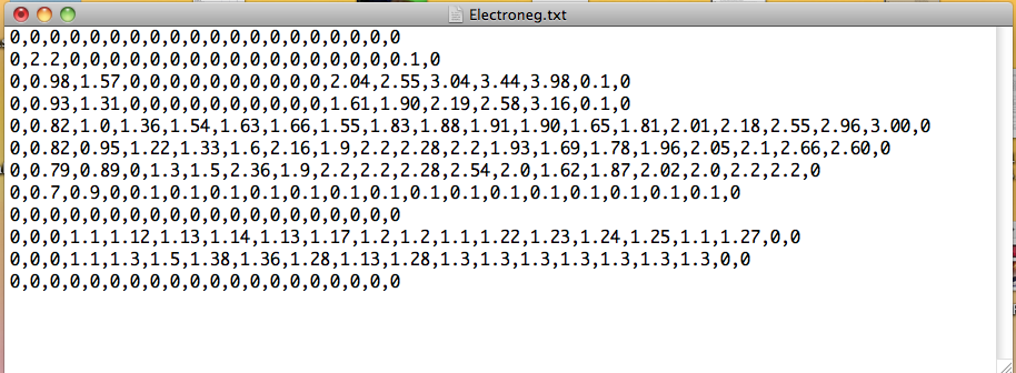
Electronegativity values typed in as comma-separated rows. Blank spaces on the chart are given zeros. The final grid is 12 rows of 20 values each.
Once the comma-separated rows of numbers are done and checked, the students save the array as a raw text file (.txt) so that all formatting is erased. They then load the file up into a program called Image J. This program is freeware developed by the National Institute of Health and is very useful for analyzing images. To load in the number array .txt file, students need to go to the file menu and choose “File-Import-Text Image” and select their .txt file. This will create a grayscale image based on the .txt values: the lowest values (the zeros around the edges of the periodic table) are black and the highest value is made white. It will be a small image since the entire array is 20 by 12 pixels. You can save the image created or zoom in on it as close as it will with Command-+ and save a screen shot of it.
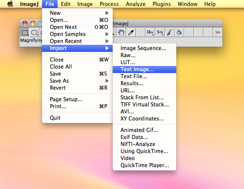
Importing the .txt file as a Text Image into Image J software

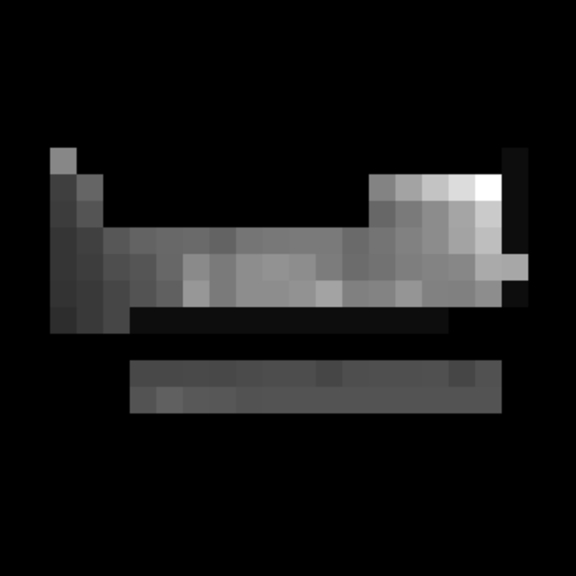
The original grayscale heightmap is only 20 x 12 pixels. You will need to zoom in and save a screen shot of the image.
In Adobe Photoshop or GIMP, students load in the screen shot and cut it so only the grayscale area remains, then increase the resolution. You will need to blur it slightly (2-3 pixel Gaussian blur) to get rid of artifacts around the edges of the squares. Then make the canvas square by adding a black background using the “Image-Canvas Size” feature in Photoshop. You can do a similar function in GIMP. Save it as an RGB or 8-bit grayscale PSD or PNG file. This prevents the grayscale heightmap from getting distorted in the 3-D terrain editor.

The grayscale heightmap in Image J after zooming in.
Now open up your favorite 3-D modeling software. I use Daz3D Bryce because it makes excellent terrains. Most other 3-D software can do terrains out of grayscale heightmaps. Some free or low cost options are Blender and Autodesk Maya (you can find a free PLE version of it). You will then need to load in the square grayscale file you just made using the “Load” buttons in the Picture tab of the Terrain Editor, smooth it, and put a texture on it.
Electronegativity heightmap after adding black edges to make it a square. This avoids distortion in the 3D modeler.
At this point you have a 3-D terrain showing the strength of a periodic property for each element. I am including several examples here. The models can be animated or have a camera fly around it. You can add lights and render out images, then put together a class powerpoint using all the student’s images to demonstrate periodicity and the Periodic Law.
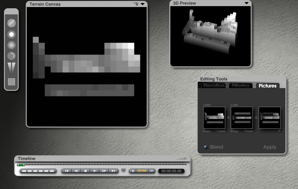
The Terrain Editor in Daz3D Bryce. The model may need additional smoothing to round off artifacts.
I’ve also put together a video that describes the history of the periodic table as narrated by Dr. Eric Scerri of UCLA. You can find it on the video page of this blog.
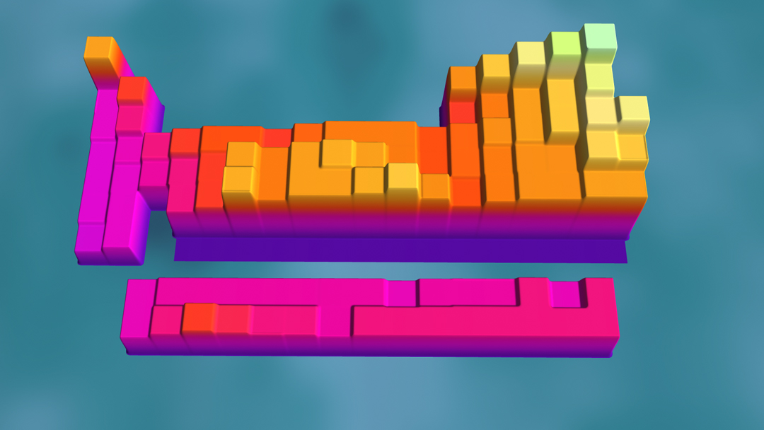
Electronegativity model in Daz3D Bryce. An altitude sensitive texture has been applied.
Give it this activity a try and let me know how it turns out. I’d love to see examples of what your students come up with.
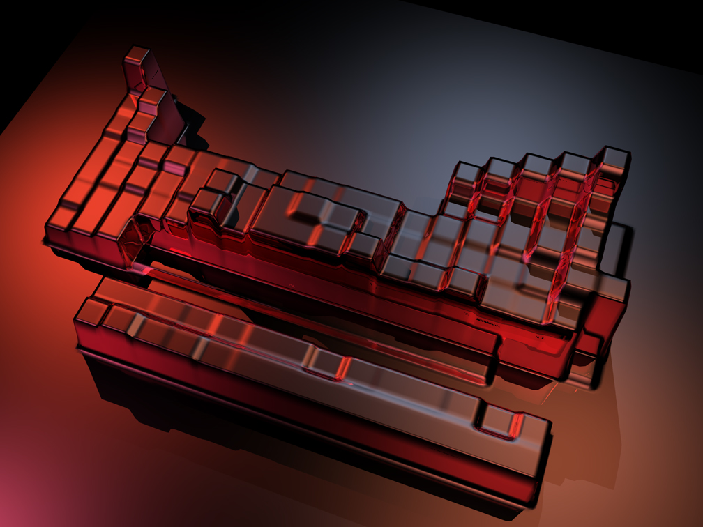
Electronegativity model in Daz3D Carrara with a little mood lighting


